Blog Posts
The checkerboard pattern started to become too basic for our fancy model.
We wanted something less regular; that’s when the texture enters.
And what’s more fun than letting the computer create the textures for you?
In fact one of our idea was to have the model stand on a wooden table, therefore we needed some sort of wood-ish texture.
Well it turns out it’s really not difficult to generate wood using procedural noise.
Fortunately for us the glm library supports simplex noise.
Here are the operations we found looked good:
- Choose one of the two coordinates and scale it by an arbitrary factor.
- Set the other coordinate to a constant value and sample a noise value at that point.
- Set the other coordinate back to its original value plus , and sample two other noise values at a various scaled displacement.
- Apply a smooth periodic function such as to with different periods, add them together and normalize the result .
- Finally blend two colors .
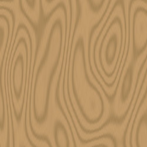
A sample of the final texture.
You will see later that with lower contrasts it’s hard to tell that it is not synthetic.
This function can thereafter be used a texture that’s computed on the fly (it’s not particularly expensive so we can allow it).
Here we decided to stick to the checkerboard by alternating with two different types of woods.
A small trick is to use a different seed for each wood type to mark the transition.
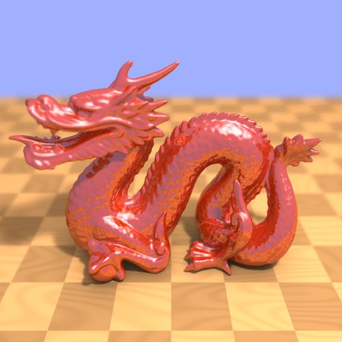
The final result, our best image so far.
Until now our materials reflected the light in all directions.
Polished materials don’t behave like that, the light is mostly reflected in a single direction.
Today we implemented more parameters that controlled this behavior.

When a ray hits a perfectly smooth surface (red), part of its energy is reflected (blue), some other part is refracted (green), and finally a little bit is absorbed (not represented).
We decided not to do refractions because we lacked time.
The reflection were fairly easy to implement.
We used a recursive function that represented a ray bouncing from triangle to triangle until it reached a maximum number of iterations or did not intersect with anything.
Given a normalized ray and a normal vector , the reflected ray may be obtained using the following relation:
We also implemented a specularity feature for shiny surfaces.
The simulated light source will appear to be reflected on the surface towards the observer.
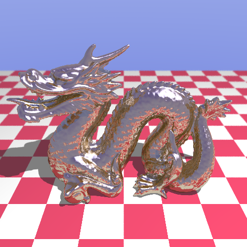
As we include more features the images become more and more realistic, such as this metallic dragon.
After completing our efficient queryable structure (and a lot of debugging!), we wanted to test our program on more complex scenes.
One of our goals was to load arbitrary models from a file.
A common file format that very simply describes a 3D model STL.
The model does not contain any color information and the description is merely just a triangle mesh: precisely what we can process.
The informations are encoded in binary in the following way:
| Data Type |
Comment |
char[80] |
Textual header |
uint32 |
The number of triangles |
Triangle[] |
The triangles |
The Triangle structure is defined as follows:
| Data Type |
Comment |
Vector |
The normal vector |
Vector[3] |
The vertices , and |
uint16 |
A checksum |
And finally Vector is defined as:
| Data Type |
Comment |
float32[3] |
The , and coordinates |
Here are the results of some of our tests with some STL models that are in the public domain:
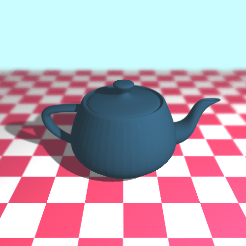
The Utah teapot on a checkerboard pattern rendered with a focus blur effect.
This scene contains around 10,000 triangles in total.
The rendering took 15 minutes with all optimizations enabled and a sampling rate of 400 rays per pixel.
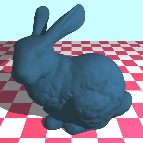
The Stanford bunny, around 87,000 triangles; rendering with a supersample (antialiasing) took 90 seconds.
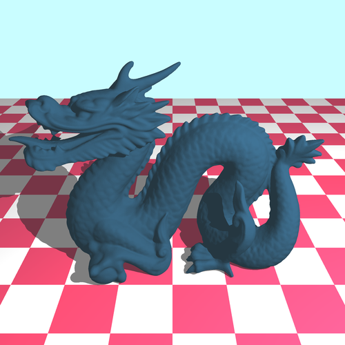
The Stanford dragon, around 300,000 triangles; rendering with the same parameters as the bunny took 120 seconds.
As you can see the complexity of the scene now barely affects the rendering time, which is an excellent news.
In this second post we will describe the actual usage of the tree.
This routine is stored in black-box function that efficiently finds the closest intersection between a ray and a triangle.
Firstly we need to define the ray-cube intersection.
Each AABB has 6 faces, we have to find the face with the closest intersection (if it exists).
As an example, let’s take one of the two faces aligned with the axis on :
Assuming the ray is not parallel to the plane, we have a single solution:
First we need to check that the point in indeed on the face and .
These properties should only hold for either 0 or 2 faces at the same time (because the cube is a convex set).
In the first case we can safely return an empty result; while in the second case the smallest value of the two should be returned.

Each square is recursively tested in-order, sorted by the distance from the closest intersection from the source of the ray.
When a leaf is reached all the line segments (the triangles in our case) are tested against the ray.
Once an intersection is found, the result is guaranted to be the closest thus the function breaks.
Now that we have our ray-cube intersection, we can build the octree collision detection function.
If the cube has children, we filter and sort them by their value of defined previously.
Then we recursively call the same function on these cubes ordered in ascending order.
If a cube returns an intersection, the iteration stops and the result is propagated back to the initial caller.
Otherwise if the cube doesn’t have any children (base case), we perform a ray-triangle intersection test with all the triangles of that node.
All the effects we previously presented are very slow with our current intersection checking routine.
In order to be able to combine them together, we would need an astronomical amount of time to generate a single frame.
Thus it was absolutely vital to improve it.
To do that we need to segment the space (a list of triangles) into smaller fragments. Several methods exist: bounding boxes, bounding spheres, etc.
We decided to work with axis aligned bounding boxes (will be further noted AABB) using an octree.
This particular orientation of the boxes is very important because it makes the computations much easier for the machine (and for us!).
The octree is a partioning system that wraps the scene inside a cube, this cube is then split into 8 smaller cubes of equal sizes that are also AABB, these smaller cubes are split again in 8 even smaller cubes, and so on until we reach an arbitrary threshold or some condition.
The idea is that the depth of the resulting tree is proportional to the logarithm of the size difference between the biggest cube and the smallest one, and a query would only require that many operations.
The code for the octree is divided into two independent steps: the construction and the querying.
In this first post we will briefly describe the construction. Note that in our case this procedure does not need to be optimal as it is only going to be run once, at the beginning.

This figure illustrate the process layer by layer in the 2D case (quadtree).
At the last step all the squares are leaves and contain at most one line segment.
As a starting point we need to find the smallest box that contains all the triangles.
This is done in a single pass and will serve as the base case of our recurrence.
The boxes can be represented by only two points, the minimum and maximum corners, and they contain a list of triangles and an optional list of boxes.
Upon splitting a cube, we would like to know which triangles intersect a cube.
A simple filter that we started with is to compute the bounding sphere of that triangle (which is nothing more than the circumscribed sphere) and then process the sphere-cube intersection (which is easier).
While this method is guaranteed to preserve all positives, it can also misclassify a lot of negatives.
Then, as long as there are two or more triangles and the threshold is not reached, the branching continues.
Hopefully the number of triangles in each child is reduced by a factor at each step.
Until now we assumed our camera to be a perfect pinhole model: the convergence area is an ideal point.
Both the eye and the camera have a mechanism to filter light, respectively the pupil and the aperture.
In practice the pinhole is always a few millimeters wide, in order to capture enough light and reduce the required exposure time.
The side effect is that all elements of the scene cannot appear crisp at the same time; typically only a single depth of field can be captured clear while the others are blurry.
It’s essentially what is meant by the term “focus”.
We are able to reproduce this phenomenon in ray tracing, with once again a stochastic sampling process.
We will introduce two additional parameters to our camera:
- the focused distance in respect to the camera
- the radius of the aperture
And of course not to mention a sampling rate.
By the way we defined our parameters, we want object located at the focused distance to appear clear.
Therefore for each pixel we will compute the point that would come out the sharpest if there happened to be an object there.

The aperture is the left black box, the chosen focus is represented by the dashed line and the three objects represented by three colored circles.
Observe that all the rays intersect on the arc, and that the only object that will render correctly is the blue one.
Let be our focal point (the position of the camera) and the normalized ray for that pixel.
We have , the focused point.
Now let’s define two variables, and .
Together they will allow us to determine the new focal point:
The last step is to sample rays passing by and different focal points on the aperture plane:
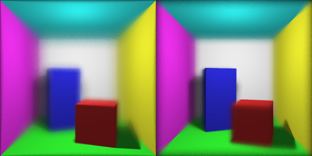
Focusing respectively the red and the blue cuboid with 100 samples per pixel
Now that we have improved the ambient component of our lighting pipeline, we will now focus on the direct lighting.
Currently the direct lighting of each virtual point falls into two case:
- the point is directly exposed to the light source, in that case the radiation formula is used
- an object obstructs the light source, then this component is zero
This simple procedure produces sharp but unreaslistic shadows.
In fact in real life the shadows appear blurry especially when the distance between the occluding object and the surface is large.
The trick we used to create this effect relied once again on sampling rays from the virtual point, but this time in the direction of the light source and with a random displacement.
The ratio between the number of ray that did not reach the light source and the total rays casted corresponds to the intensity of the shadow.
Unfortunately the task of randomly (and uniformly) displacing a ray is less trivial to accomplish.
However it turns out we can use another trick that relies on the fact that for small angles.
This property can be exploited in our case; the displacement would be a small vector bounded by a cube that gets added to the normalized vector pointing towards the light source.
Since the displacement is expected to be very small, the error would be virtually unnoticeable.
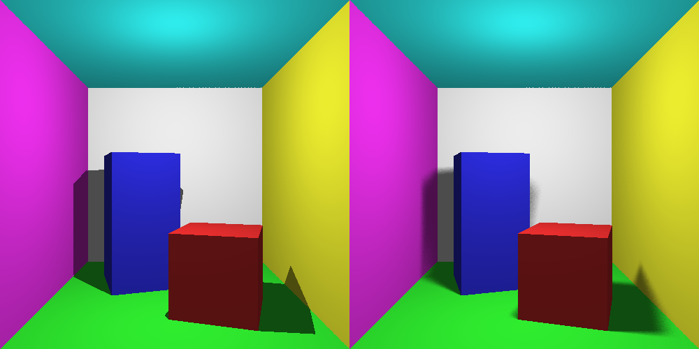
Hard shadows on the left figure and soft shadows on the right (100 samples per pixel)
During our experiments we encountered artifacts near the edges (the left shadow on the figure incorrectly appears brigther in the corner).
We are not quite sure yet what is causing them, we are suspecting floating point precision issues but that’s only speculative.
As explained in the previous post, computing light bounces is an expensive operation.
Fortunately we can achieve a closely accurate result using the ambient occlusion technique.
The principle is rather simple, it comes from the observation that closed spaces such as concave corners tend to be darker than convex areas.
Moreover this is applies indepently from the position of the light source (on a relative scale).
This assumption is quite fair in the sense that open areas are likely to be more exposed to the light.
The “openness” of an area is determined by integrating the bounded rays over the hemisphere at that point, divided by the total area of the hemisphere.
The hemisphere is oriented outwards in respect to the normal vector.
The radius of the hemisphere is an arbitrary value that corresponds to the local area that must be considered.
Larger values create more realistic renderings but are possibly also more expensive.

The point of interest is represented in magenta. The hemisphere orientation is determined by the normal vector of the surface (n). The sampled rays are in blue and red depending on wether they intersected in a surface or not. The green area is the sought area
Now the question arises on how to implement such a procedure.
Since it is an improvement on the regular ambiant lighting system we updated this function such that instead of returning a constant value it would be affected by the position of the intersection.
The integral can be approximated using a stochastic sampling process: we will cast random rays and sum their results.
The trick used to generate a random vector in a sphere is to first generate a random vector in a cube (trivial), and discard it if its norm is greater than one.
Finally if the scalar product between the vector and the normal is negative that means it is not in the hemisphere, so the opposite vector is chosen instead.
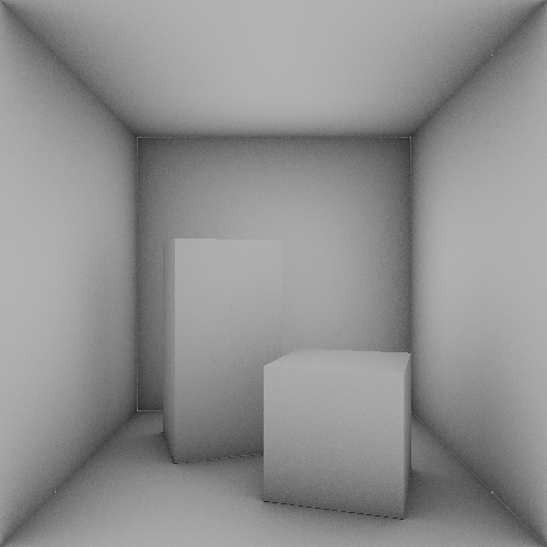
Scene rendered without colors and only ambient occlusion; radius was set to 1 distance unit and sampling to 300 rays per pixel
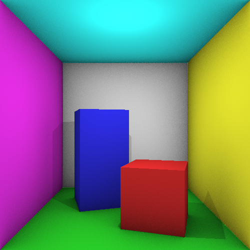
The same scene with the previous effects
The results are quite encouraging, even though the rendering time has drastically increased (the previous images took half an hour to complete).
As we are working on implementing an efficient queriable structure for the scene, we are confident that this issue will be solved or at least greatly reduced when we merge the two.
In fact it would be fairly easy to first filter out all the triangles that are out range before doing the sampling process.
The main focus of our project was to improve the raytracer from the lab. We will focus on the following main tracks:
-
Scene representation
Currently the rendering is very slow, the main reason being that the intersection pipeline is not optimal.
Each time such an intersection is computed, all the triangles of the scene are checked.
This can greatly be improved by segmenting the space and cutting expensive operations by only checking triangles that are possibly intersecting.
Therefore we are planning to implement an octree of triangles, aswell as some other optimization strategies.
-
Better shading and lighting
The current light simulation is rather basic and only allows the existence of binary shadows.
In reality the movement of light is more complex than a direct exposition, in fact the photos generally bounce in another direction when hitting a surface.
Thus to create a realistic simulation it’s not sufficient to only consider the direct light.
In practice simulating bounces is an exponentially complex problem.
In this project we will try different techniques that approximate this effect such as ambiant occlusion and light tracing.
We might aswell consider simulating other phenomena like reflexion and refraction on different materials, distance blur, fog…
In addition to that, we plan to include some of the following minor features:
- Loading scenes from a file, in some possibly custom format
- Antialiasing
- Allow triangles to hold a bitmap texture instead of a single color
- Possibility of rendering a sequences of images with a moving camera
We are two students at KTH, Florian and Martin.
In this blog we are going to describe the process and the making of our project in Computer Graphics and Interaction.
We will post regular updates in a hopefully nearly daily basis of our current progress.
Stay tuned!